Periodic Autoencoder - Explanation and Addendum
In DeepPhase we use a Periodic Autoencoder (PAE) to learn periodic features from data. In particular, we aim to extract a small number of phase values that well-capture the (non-linear) periodicity of higher dimensional time series data. If you are solely interested in implementing the Periodic Autoencoder for your use case look for the supplementary material in the ACM Digital Library. What follows is a brief explanation of how we can extract phase features from data.
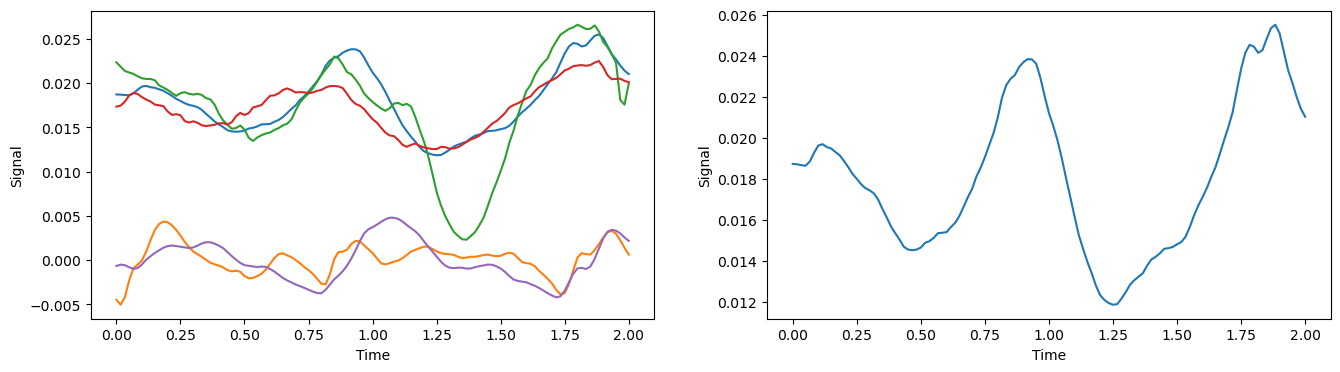
Given some number of temporal signals, which are assumed to have some joint periodicity, the Periodic Autoencoder learns a latent space, $\mathbf{L}$, with a few (say 5) latent signals of the same length as the original signals. These latent signals might look something like the signals in the left plot below. For each one of these signals we then aim to extract a good phase offset that captures its current location as part of a larger cycle.
However, any one of these signals (say the blue curve in the right plot) may not have a single obvious frequency, amplitude, or phase offset. So the question becomes, what is a good way to calculate a phase value for such a curve?
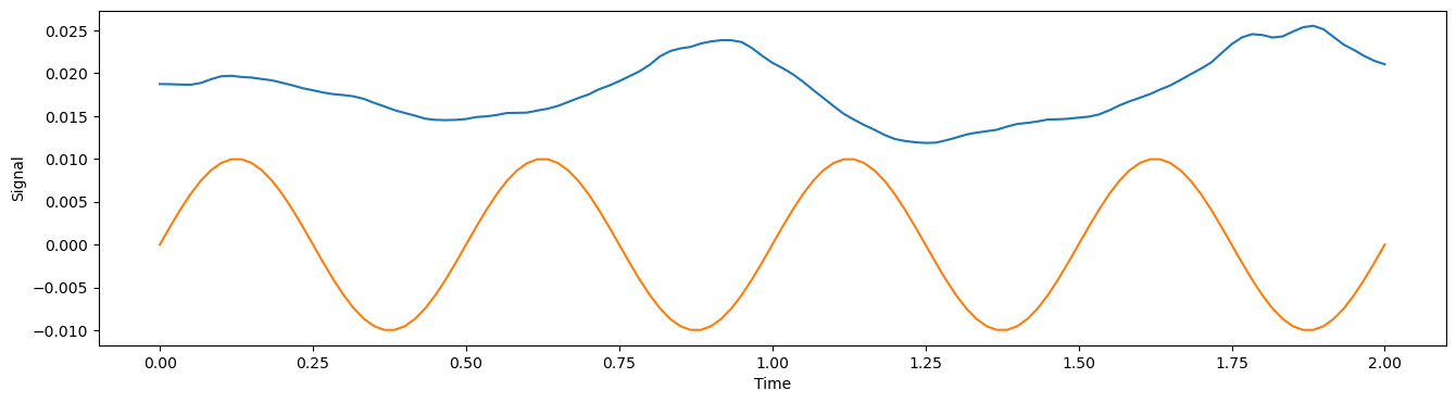
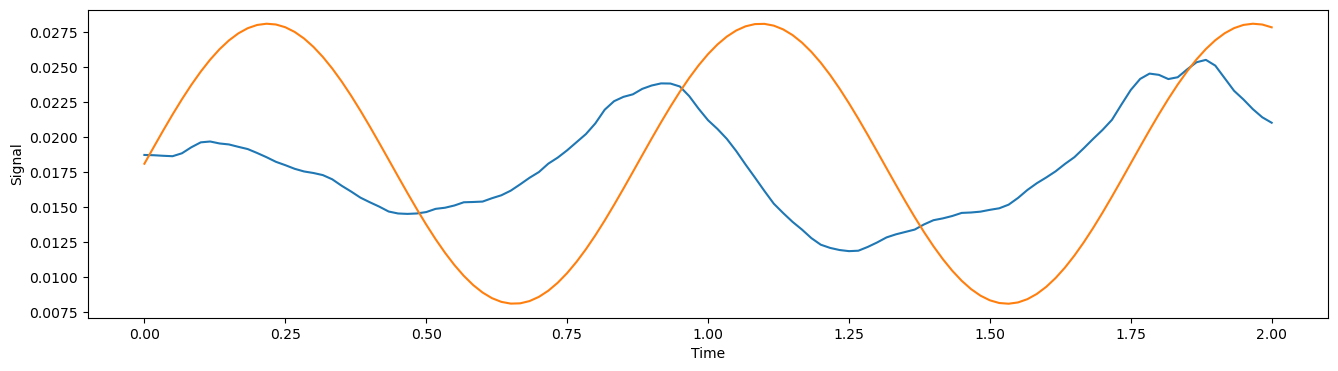
The approach taken with the Periodic Autoencoder is to approximate each latent signal with a sinusoidal function $\Gamma(x) = A sin (2 \pi (Fx - S)) + B$, parameterized by $A$, $F$, $B$ & $S$, and to then use $S$ as the phase offset. The plot below shows the same blue curve from above along with the function $\Gamma(x) = 0.01 sin(4 \pi x)$. Our aim is to better set the parameters of $\Gamma$ such that the orange curve more closely approximates the blue curve. After calculating these sinusoidal functions for all latent signals the PAE then aims to reconstruct the original data from these functions. This places a big inductive bias on the latent space that assumes a few periodic functions will be sufficient for reconstruction.
So, to find the parameters for $\Gamma$, let’s say this $1D$ signal (blue curve) contains $N$ points over a time window of $T$ seconds, then after applying a real discrete Fourier transform [1] we receive $K+1$ Fourier coefficients $\mathbf{C}=[c_0, c_1, \dots, c_K]$ where $K = \left\lfloor\frac{N}{2}\right\rfloor$. These coefficients correspond to frequency bins centered at $\mathbf{f}=[0, 1/T, 2/T, \dots, K/T]$ Hz (the real DFT does not calculate the negative frequency terms as they are redundant for real-valued signals, returning only a single-sided spectrum).
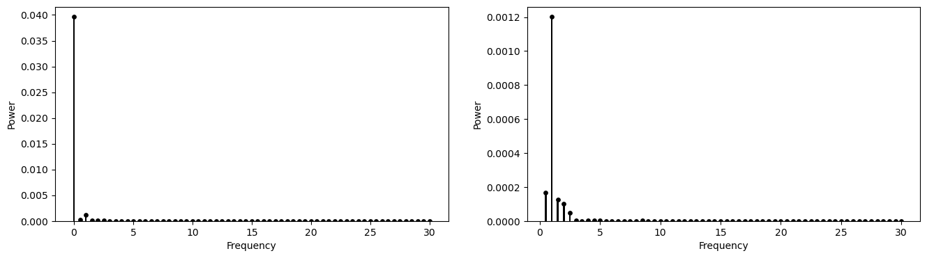
The magnitudes of the coefficients, $\mathbf{m} = [m_0, m_1, \dots, m_K]$ $= [|c_0|, |c_1|, \dots, |c_K|]$, represent the relative presence of each of the frequency bins in the signal. From this we can calculate the power spectrum (the amount of the signal’s power present in each of the frequency bins) as $\mathbf{p} = [p_0, p_1, \dots, p_K] =\frac{2}{N} [\frac{1}{2} m_0^2, m_1^2, \dots, m_K^2]$. Note that every term except the $m_0$ term is doubled since the real DFT returns the single-sided spectrum and we still wish to account for the power in the double-sided spectrum [2]. Below we show the whole single sided power spectrum in the left plot and the power spectrum without the zero frequency bin in the right plot.
$c_0$ is the “zero frequency” Fourier coefficient, which is equivalently the sum of the $N$ samples and is always real. Therefore, dividing by the number of samples gives us the mean offset of the signal which we use as the offset for the sinusoidal approximation $\Gamma$:
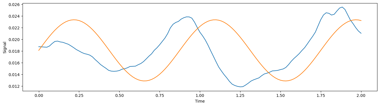
\[B = \frac{c_0}{N}.\]After applying this value of $B$, we see our approximation becomes more well aligned along the y-axis.
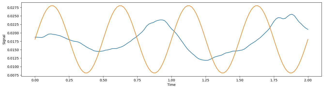
A good value for the single frequency $F$ is the mean frequency of the overall signal. We can calculate the mean frequency by taking an average of the frequency components weighted by the power with which they appear in the signal [3]. Note that the zero frequency term is not included as this is already captured by $B$.
\[F = \frac{\sum_{j=1}^K \mathbf{f}_j \mathbf{p}_j}{\sum_{j=1}^K \mathbf{p}_j}.\]After applying this $F$ with our already found $B$, we get closer to approximating the signal.
Now that the bias and frequency are accounted for, we aim to set the amplitude parameter $A$. We set $A$ such that the average power of the signal is maintained. Since we create a sine curve with a single frequency $F$, we set the amplitude such that the power in this frequency bin equals the average power of the signal $\frac{\sum_{j=1}^K \mathbf{p}_j}{N}$. A single sided power spectrum has values at height $\left(\frac{A}{\sqrt{2}}\right)^2$, [2], so rearranging we find,
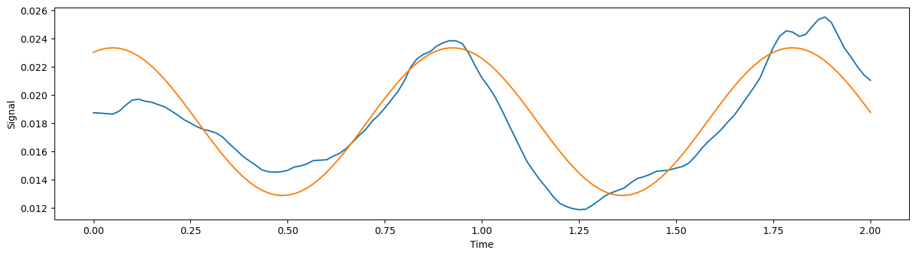
\[A = \sqrt{\frac{2}{N}\sum_{j=1}^K \mathbf{p}_j}.\]Adding this value of $A$ to $\Gamma$, our approximation gets closer again.
Finally we aim to find $S$. For signals that are not exactly periodic over the time window, we will see discontinuities in the phase extracted from the DFT. To avoid discontinuities in the PAE we learn a 2D phase representation, $(s_x, s_y)$, with a small neural network, from which we calculate $S$ as
\[S = arctan2(s_y, s_x).\]After including $S$ as the final parameter for $\Gamma(x) = A sin (2 \pi (Fx - S)) + B$, we can see that we have a reasonable approximation of our original signal.
By performing this parameterization process fully differentiably, the PAE encoder is encouraged to extract latent features which remain useful for reconstructing the original data after undergoing this severe dimensionality reduction (to 5 parameters ($F$, $A$, $B$, $s_x$, $s_y$) per latent curve). Intuitively, this means the phase representation must capture a lot of “information” about the current state of the original time series data within the available context.
Addendum
In the final figure the phase value was actually calculated with the following equations (thanks to Mario Geiger). You may have some luck replacing the small phase learning network with these operations, but I haven’t had time to check that it is well behaved in practical applications.
\[s_x = \sum_{i=1}^{N}(y_i - B) cos(2 \pi F x_i)\] \[s_y = \sum_{i=1}^{N}(y_i - B) sin(2 \pi F x_i)\] \[S = arctan2(s_y, s_x)\]Where ${(x_i, y_i)}$ are the $N$ samples that make up our signal (blue curve). With these values we find our approximation (orange curve) with:
\[A cos(2 \pi F x - S) + B .\]Code
The figures in this post were generated with this short python script.
There is a basic implementation of the Periodic Autoencoder in the supplementary material files here.